Draw a Filled-in Circle Mathematica

Preface

---

This section addresses a buitiful application of Mathematica to plot figures with fillings. Therefore, this department presents numerous examples.

Return to computing page for the first course APMA0330
Return to computing folio for the second class APMA0340
Render to Mathematica tutorial for the first form APMA0330
Return to Mathematica tutorial for the second course APMA0340
Render to the chief folio for the grade APMA0330
Return to the chief folio for the course APMA0340
Return to Function I of the course APMA0330

Plotting with filling

---

		We repeat the previously considered example for a piecewise linear role with filling: Plot[2 - 2*ten, {x, 0, ane}, FillingStyle -> Light-green, Filling -> Bottom]
Piecewise linear function		Mathematica code

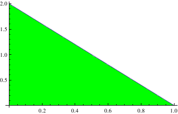		Now we change the colour of filling: Plot[2 - 2*x, {ten, 0, 1}, FillingStyle -> Green, Filling -> Bottom]
Example of green color filling.		Mathematica code

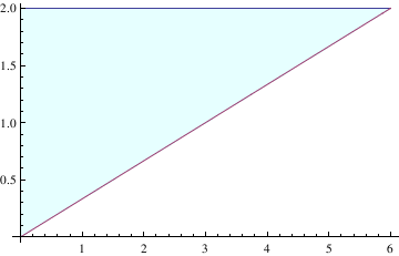		Now we change the colour of filling: Plot[{2, (x/3)}, {x, 0, 6}, Filling -> {one -> {ii}}, FillingStyle -> LightCyan]
Example of light cyan color filling.		Mathematica code

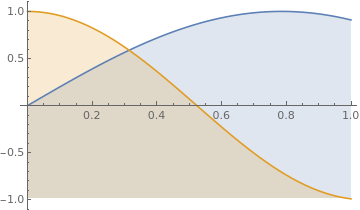
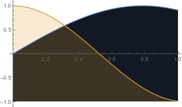		This specifies a specific filling to be used only for the showtime curve. Plot[{Sin[2*x], Cos[3*ten]}, {x,0,1}, Filling -> {ane -> 0.5}]
Ii curves with singled-out fillings.		Mathematica code

		Plot[{Sin[2*10], Cos[iii*x]}, {x, 0, 1}, Filling -> Bottom]
Region between sine and cosine functions.		Mathematica lawmaking

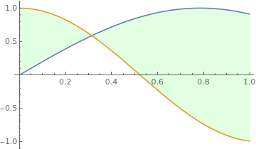		Some other color of filling: Plot[{Sin[2*x], Cos[3*10]}, {x, 0, 1}, Filling -> {ane -> {2}}, FillingStyle -> LightGreen]
Region betwixt sine and cosine functions.		Mathematica code

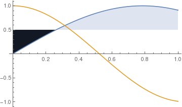		This code specifies a specific filling to be used just for the first bend. Plot[{Sin[2*ten], Cos[3*ten]}, {x,0,1}, Filling -> {1 -> 0.5}]
Simply i part of the region is specified.		Mathematica lawmaking

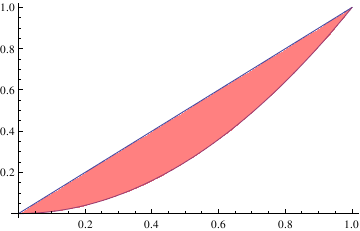		Plot[{10, x^ii}, {10, 0, ane}, Filling -> {one -> {two}}, FillingStyle -> Pinkish]
Region betwixt 2 curves.		Mathematica lawmaking

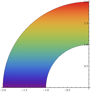
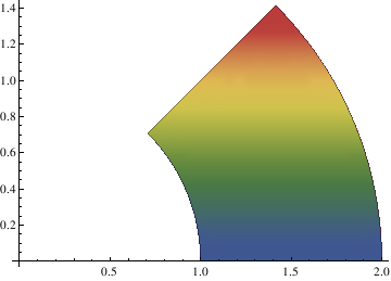		At present we modify the colour of filling: Bear witness[PolarPlot[{i, 2}, {t, 0, Pi/four}], RegionPlot[ 10^2 + y^2 >= 1 && ten^2 + y^2 <= 4 && y/ten <= 1, {10, 0, 2}, {y, 0, 2}, ColorFunction -> "DarkRainbow"]]
Example of PolarPlot.		Mathematica code

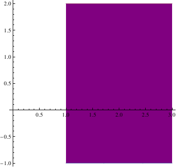		Plot[{-1, 2}, {x, 1, 3}, Filling -> {i -> {ii}}, FillingStyle -> Purple, AspectRatio -> Automated, AxesOrigin -> {0, 0}]
Rectangle.		Mathematica code

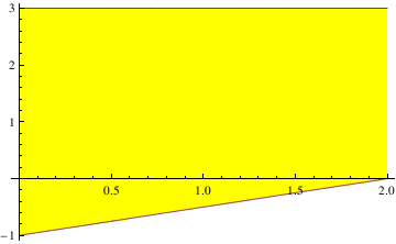		Plot[{three, (ten/ii) - one}, {x, 0, 2}, Filling -> {one -> {2}}, FillingStyle -> Yellow]
Figure with filling.		Mathematica code

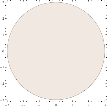		RegionPlot[{x^2 + y^ii <= 9}, {x, -three, 3}, {y, -3, 3}, PlotStyle -> LightBrown]
Figure with filling.		Mathematica code

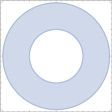
		Show[PolarPlot[{one, two}, {t, Pi/two, Pi}], RegionPlot[x^two + y^two >= 1 && ten^2 + y^2 <= 4, {x, -two, 0}, {y, 0, 2}, ColorFunction -> "Rainbow"]]
Part of a circumvolve with filling.		Mathematica code

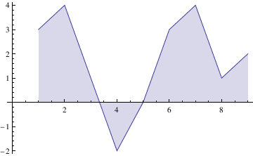
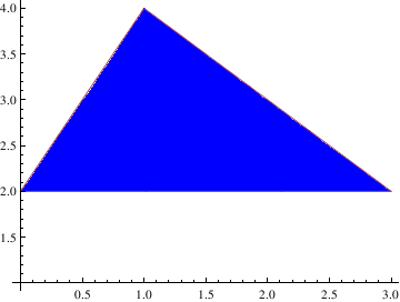		To lift a traingle over the horizontal axis, type: tr = Plot[{1., Max[one, Min[two ten + 1, 4 - x]]}, {ten, 0, 3}, AspectRatio -> i/2, Ticks -> {{0, 1, 2, 3}, {0, 1, ii, 3}}, Filling -> Axis, FillingStyle -> Blue, Axes -> True, AxesStyle -> Directive[Thick]] a = Graphics[{{Opacity[0], White, tr[[1]]}, GeometricTransformation[{Opacity[i], Bluish, tr[[i]]}, TranslationTransform[{0, ane}]]}] Show[a, Axes -> True, AxesStyle -> Black, AspectRatio -> 0.75]
Triangle is lifted over the centrality.		Mathematica code

RegionPlot[Sin[x y] > 0, {x, -1, 1}, {y, -1, 1},
FrameTicksStyle -> Directive[FontOpacity -> 0, FontSize -> 0]]

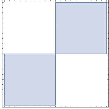
When plotting, you still see frameticks data:

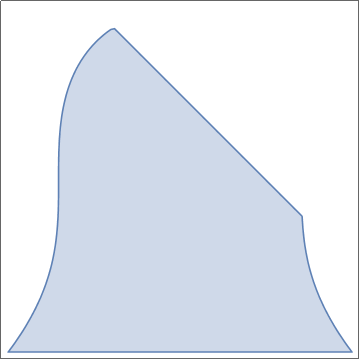
rp = RegionPlot[x^ii + y^three/four < 2 && x + y < i, {x, -2, 2}, {y, -2, 2}, FrameTicks -> Automated]

First extract the frameticks information and change the labels to blank:

newticks = Final@Commencement[AbsoluteOptions[rp, FrameTicks]];

While Mathematica complains nigh that Ticks: {Automatic,Automatic} is not a valid tick specification, information technology notwithstanding does its job. next nosotros type:

Evidence[rp, FrameTicks -> newticks]

You may as well try

newticks = Last@Start[AbsoluteOptions[rp, FrameTicks]];
newticks[[All, All, 2]] = "";

but Mathematica will complain again and out will be the same.

RegionPlot[1 < Abs[ten + I y] < 2, {x, -2, 2}, {y, -2, 2}, ImagePadding -> 1]

		Another example: Graphics3D[{Texture[img], EdgeForm[], Cylinder[{{0, 0, 0}, {0, 0, ii Pi}}, one]}, Boxed -> False]
Two pieces of a circumvolve.		Mathematica lawmaking

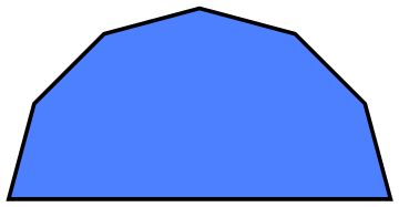
We plot half of the polygon:

poly = Polygon[Table[North[{Cos[due north *Pi/half-dozen], Sin[n*Pi/half dozen]}], {northward, 0, 6}]]
Graphics[{RGBColor[0.3, 0.5, ane], EdgeForm[Thickness[0.01]], poly}]

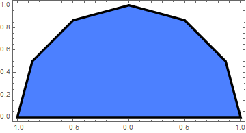
Evidence[%, Frame -> True]

Parametric Plots with fillings

---

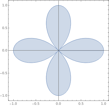
		ParametricPlot[ Cos[two theta] {Cos[theta], Sin[theta]} r, {theta, 0, 2 Pi}, {r, 0, 1}, Mesh -> Imitation, PlotPoints -> {30, 2}]
Iv cusp curve r = cos(2 θ).		Mathematica code

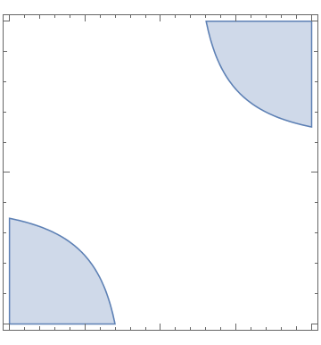
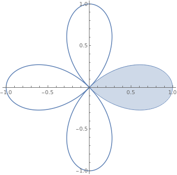
		g1 = PolarPlot[Cos[two theta], {theta, Pi/four, 2 Pi - Pi/iv}]; g2 = ParametricPlot[ Cos[two theta] {Cos[theta], Sin[theta]} r, {theta, -Pi/4, Pi/4}, {r, 0, one}, Mesh -> False]; Show[g1, g2, PlotRange -> All]
Function of the curve r = cos(2 θ).		Mathematica code

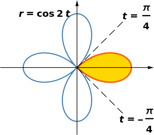
		txt[t_, {x_, y_}] := Fashion[Text[t, {10, y}], FontSize -> 30, FontWeight -> Assuming] {xmin, xmax} = {-ane.425, i.425}; {ymin, ymax} = {-1.25, ane.25}; PolarPlot[Cos[2 t], {t, 0, 2 Pi}, PlotRange -> {{xmin, xmax}, {ymin, ymax}}, PlotStyle -> {ColorData["Legacy", "SteelBlue"], Thickness[0.007]}, Ticks -> None, Epilog -> {Inset[ RegionPlot[(x^2 + y^ii)^(3/ii) <= ten^2 - y^2, {10, -0.02, one}, {y, -i, i}, PlotStyle -> ColorData["HTML", "Golden"], BoundaryStyle -> Directive[Thickness[0.025], ColorData["Legacy", "CadmiumOrange"]], Frame -> False, AspectRatio -> Automated, ImageSize -> 2.6*72], {0.5, 0}], Black, Thick, Dashing[{0.045, 0.03}], Line[{{0, 0}, {0.85, 0.85}}], Line[{{0, 0}, {0.85, -0.85}}], Dashing[{}], Thick, Pointer[{{xmin, 0}, {xmax, 0}}], Arrow[{{0, ymin}, {0, ymax}}], txt[TraditionalForm[HoldForm[r == cos 2 t]], {-0.vi, one.0}], txt[TraditionalForm[HoldForm[t == Pi/iv]], {1.125, 0.925}], txt[TraditionalForm[HoldForm[t == -Pi/4]], {ane.125, -0.99}]}, ImageSize -> seven*72]
One cusp from the curve r = cos(two θ).		Mathematica code

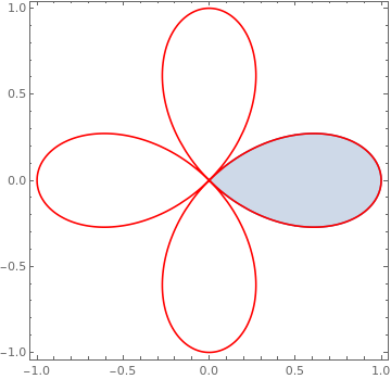
		Another version: Show[{RegionPlot[(x^2 + y^2)^(1/ii) <= Cos[2 ArcTan[y/x]], {ten, 0, 1}, {y, -i/2, 1/ii}], PolarPlot[Cos[2 theta], {theta, 0, ii Pi}, PlotStyle -> Red]}, PlotRange -> All] or Show[{RegionPlot[(x^2 + y^ii)^(3/2) <= x^2 - y^2, {x, 0, 1}, {y, -1/ii, i/2}], PolarPlot[Cos[ii theta], {theta, 0, 2 Pi}, PlotStyle -> Red]}, PlotRange -> All] or PolarPlot[Cos[ii theta], {theta, 0, 2 Pi}, PlotStyle -> Red, Prolog -> RegionPlot[(ten^ii + y^ii)^(3/2) <= x^ii - y^2, {10, 0, ane}, {y, -1/2, 1/2}][[i]]] or s = PolarPlot[Cos[2 theta], {theta, 0, two Pi}]; s1 = PolarPlot[Cos[two theta], {theta, -Pi/4, Pi/four}] /. Line -> Polygon; Evidence[s, s1]
1 cusp from the curve r = cos(ii θ).		Mathematica code

Polar plots with fillings

---

I fashion to go around a problem to make plots with filling is to use ParametricPlot

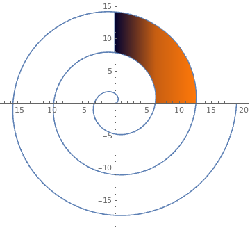
		parmplot = ParametricPlot[ r {Cos[t], Sin[t]}, {t, 0, Pi/2}, {r, 2 Pi + t, 4 Pi + t}, ColorFunction -> "RustTones"]; Show[ParametricPlot[t {Cos[t], Sin[t]}, {t, 0, 6 Pi}], parmplot]
Archimede's spiral.		Mathematica code

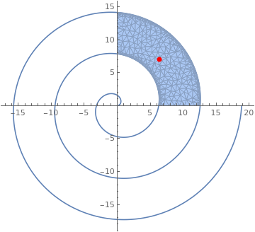
		cartreg = ImplicitRegion[ 2 \[Pi] < Sqrt[x^2 + y^2] - ArcTan[x, y] < 4 \[Pi] && 0 <= x <= 15 && 0 <= y <= 15, {x, y}]; regiontoplot = DiscretizeRegion[cartreg, AccuracyGoal -> five]; NumberForm[#, {8, v}] &@Area[regiontoplot] NumberForm[Integrate[1, {10, y} \[Element] regiontoplot], {8, v}]; pt = RegionCentroid[regiontoplot]; Show[ParametricPlot[t {Cos[t], Sin[t]}, {t, 0, 6 Pi}], regiontoplot, Graphics[{PointSize[Large], Red, Indicate[pt]}]]
Archimede'due south spiral with a dot.		Mathematica lawmaking

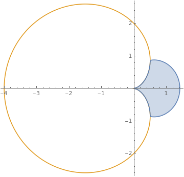
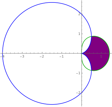
		Show[PolarPlot[ Evaluate[{{1, -ane} Sqrt[ii Cos[t]], 2 (one - Cos[t])}], {t, -\[Pi], \[Pi]}], RegionPlot[ Sqrt[x^2 + y^ii] > 2 (i - Cos[ArcTan[x, y]]) && Sqrt[ten^two + y^ii] < Re@Sqrt[2 Cos[ArcTan[10, y]]], {x, -ii, 2}, {y, -3, iii}], PlotRange -> All]
Shading between polar graphs.		Mathematica code

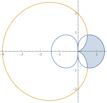
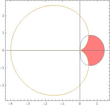
		Another plot: Show[PolarPlot[{Sqrt[2 Abs[Cos[t]]], 2 (1 - Cos[t])}, {t, -\[Pi], \[Pi]}], RegionPlot[ four (ane - Cos[t])^2 < r^ii < 2 Cos[t], {r, 0, three}, {t, -Pi, Pi}, PlotPoints -> 30] /. GraphicsComplex[a_, b__] :> GraphicsComplex[#1 {Cos[#2], Sin[#2]} & @@@ a, b]]
Shading between polar graphs.		Mathematica code

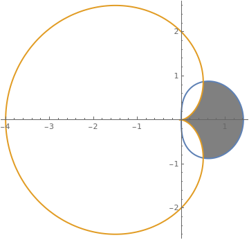
		Using Cartesian coordinates: eqns[t_] := {Sqrt[2 Cos[t]], 2 (1 - Cos[t])}; region = PolarPlot[Evaluate@eqns[t], {t, -\[Pi], \[Pi]}, RegionFunction -> Role[{x, y, t, r}, {#ane > #ii} & @@ Re[eqns[t]] // Get-go]]; pts = Cases[region, Line[x___] :> x, Infinity]; colors = {Darker@Green, Bluish}; Show[PolarPlot[Evaluate@eqns[t], {t, -\[Pi], \[Pi]}, PlotStyle -> colors], ListLinePlot[pts, PlotStyle -> colors, Filling -> Axis, FillingStyle -> Purple], PlotRange -> All]
Shading between polar graphs.		Mathematica code

		Yous can parameterize your polar functions on to discs, and then shade appropriately. \[Rho][t_] := Sqrt[2 Cos[t]]; \[Sigma][t_] := ii (1 - Cos[t]); ParametricPlot[{{r Cos[t] \[Rho][t], r Sin[t] \[Rho][t]}, {r Cos[t] \[Sigma][t], r Sin[t] \[Sigma][t]}}, {t, -\[Pi], \[Pi]}, {r, 0, i}, PlotStyle -> {{Opacity[.5], Reddish}, {Opacity[i], White}}, Mesh -> None, PlotRange -> All]
Shading between polar graphs.		Mathematica lawmaking

		Some other version: dt = Pi/99; pts = Join[ Tabular array[2 (ane - Cos[t]) {Cos[t], Sin[t]}, {t, 0, -Pi/iii + dt, -dt}], Table[Sqrt[2 Cos[t]] {Cos[t], Sin[t]}, {t, -Pi/3, Pi/3, dt}], Table[ii (1 - Cos[t]) {Cos[t], Sin[t]}, {t, Pi/3, dt, -dt}]]; PolarPlot[{Sqrt[2 Cos[t]], 2 (1 - Cos[t])}, {t, -\[Pi], \[Pi]}, Prolog -> {Gray, Polygon[pts]}, PlotStyle -> Thick]
Shading betwixt polar graphs with contours.		Mathematica code

Filling circles can be plotted using Graphics cammand. Graphics are represented equally symbolic expressions, using
either"directives" or "styles":

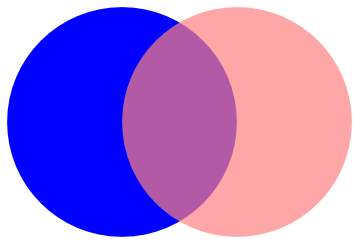
Graphics[{Blue, Disk[{0, 0}], Opacity[0.7], Pink, Disk[{1, 0}]}]

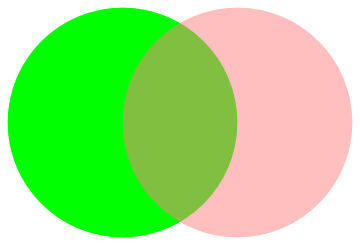
Graphics[{Mode[Disk[{0, 0}], Greenish], Opacity[0.5], Pink, Deejay[{1, 0}]}]

We tin plot Venn diagrams using the following subroutine

VennDiagram2[n_, ineqs_: {}] :=
Module[{i, r = .6, R = ane, five, grouprules, x, y, x1, x2, y1, y2, ve},
five = Table[Circle[r {Cos[#], Sin[#]} &[ii Pi (i - one)/due north], R], {i, north}];
{x1, x2} = {Min[#], Max[#]} &[ Flatten@Replace[five, Circumvolve[{xx_, yy_}, rr_] :> {20 - rr, xx + rr}, {1}]];
{y1, y2} = {Min[#], Max[#]} &[ Flatten@Replace[v, Circle[{xx_, yy_}, rr_] :> {yy - rr, yy + rr}, {1}]];
ve[x_, y_, i_] := v[[i]] /. Circle[{xx_, yy_}, rr_] :> (x - xx)^ii + (y - yy)^two < rr^2;
grouprules[x_, y_] = ineqs /. Tabular array[With[{is = i}, Subscript[_, is] :> ve[ten, y, is]], {i, n}];
Show[If[MatchQ[ineqs, {} | False], {}, RegionPlot[grouprules[x, y], {ten, x1, x2}, {y, y1, y2}, Axes -> False]],
Graphics[v], PlotLabel -> TraditionalForm[Supplant[ineqs, {} | Imitation -> \[EmptySet]]], Frame -> Faux]]

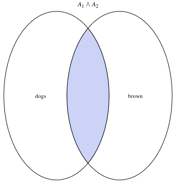
Then we plot two Venn diagrams:

a12 = VennDiagram2[2, Subscript[A, 1] && Subscript[A, 2]]
a1 = Graphics[Text[dogs, {-0.9, 0}]]
b1 = Graphics[Text[brown, {0.9, 0}]]
Evidence[a12, a1, b1]

or

a32 = VennDiagram2[2, Not[Subscript[A, 1]] && Subscript[A, 2]]
a33 = VennDiagram2[2, Non[Not[Subscript[A, 1]] && Subscript[A, ii]]]

Return to Mathematica folio
Return to the primary page (APMA0330)
Return to the Role 1 (Plotting)
Return to the Part 2 (Kickoff Order ODEs)
Return to the Part 3 (Numerical Methods)
Render to the Part 4 (Second and Higher Gild ODEs)
Return to the Part 5 (Series and Recurrences)
Return to the Part 6 (Laplace Transform)
Return to the Office vii (Purlieus Value Problems)

brownpondne80.blogspot.com

Source: https://www.cfm.brown.edu/people/dobrush/am33/Mathematica/ch1/venn.html

Share this post